Interacting with Geospatial Data in QGreenland Core

Note

QGreenland users will learn through experience that there is very often more than one way to complete a desired task in the QGIS platform

Spatial Data Overview

There are two main basic kinds of GIS data layers: vector and raster.

Vector Data

Vector data are composed of points, lines, and polygons and represent discrete features. Examples of vector data are cities (points), roads and highways (lines), and geographic boundaries like country borders (polygons) (Fig. 4). All of the vector layers in QGreenland are GeoPackage (.gpkg) files. A GeoPackage is just a platform-independent file type for storing geospatial data.

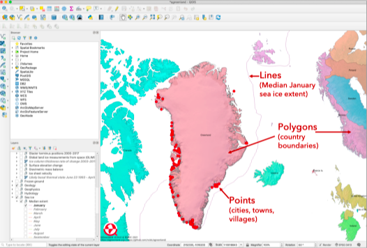
Fig. 4 Examples of vector data layers in QGreenland Core: points (towns and settlements), lines (median January sea ice extent), and polygons (country boundaries).

Vector Data Attributes

All QGIS vector data layers have associated attributes, or characteristics of the discrete features. Attributes can be almost anything: city name, road type (highway, paved, unpaved, etc.), land elevation value, population density, date, etc. The attributes of a data layer can be viewed in tabular form by right clicking on the layer in the Layers Panel and selecting Open Attribute Table from the menu options, or by clicking on the layer in the Layers Panel and then clicking on the Open Attribute Table button in the Attributes Toolbar. This opens up an Attribute Table, where the columns are the various fields, or attributes, and the rows are individual features. Clicking on and highlighting records in the Attribute Table will also highlight those specific points, lines, or polygons in the Map View. Right-click any cell to Zoom to feature, Pan to feature, or Flash feature.

Raster Data

Raster data are composed of grid cells or pixels, where each grid cell has its own value. Rasters represent continuous data, such as land elevation, surface temperature, land cover, etc. (Fig. 5). The resolution, which is the length of the grid cell sides of each raster dataset in QGreenland, is indicated in the name of the dataset, e.g.: “Ice Sheet Velocity (500 m)”. Raster layers in QGreenland are all GeoTIFF files, which are images with geographic features, such as geospatial metadata and overviews/tile pyramids.

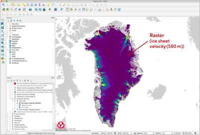
Fig. 5 Example of a Raster data layer in QGreenland, ice sheet velocity, where each grid cell in the raster is 500 m x 500 m and is color-coded by a velocity

Layer Properties

Right clicking on a data layer in the Layers Panel and selecting Properties, or simply double clicking on a layer in the Layers panel will bring up the Layer Properties dialog window, which contains a variety of information about a layer (Fig. 6). The information is organized into sections (or tabs) that can be accessed by clicking on an individual tab (e.g., Symbology) in the left sidebar of the window. The tabs listed in a vector Layer Properties dialog window differ slightly from those listed for a raster layer. The tabs most relevant to a novice QGIS user and that exist for both vector and raster layers are:

• Information: This section summarizes information about a layer, including its name, coordinate reference system, spatial extent (geographic boundaries), description (abstract), and more.

• Symbology: Every QGreenland data layer has a predefined symbology, or visual representation in the map view. See section 5.4: Editing Layer Symbology for instructions on how to modify or customize a layer’s symbology.

• Metadata: Metadata is essentially “data about data”. In QGIS, layer metadata is information about the data in the layer, including its name, description, citation, and link to the source that the data was retrieved from. As outlined in Licensing, Citing, and Contributing, published works produced using QGreenland are required to cite each dataset used in the work. Users can thus simply copy a layer’s citation directly from its metadata. An abbreviated version of a layer’s metadata can also be viewed by selecting a layer in the Layers panel and hovering your mouse over the layer name.

Note

The QGreenland team has in a few instances included comments on ‘Noted Data Issues’. Read about ‘Noted Data Issues’ in the layer metadata. These are currently noted for the ‘Populated places’ layer. Regardless, QGreenland makes no guarantees about the accuracy and validity of data contained in QGreenland. See our Disclaimer for more information.

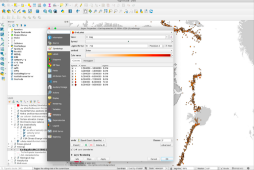
Fig. 6 The Layer Properties dialog window for the QGreenland ‘Earthquakes’ data layer.

Coordinate Reference System (CRS)

Coordinate Reference Systems (CRS), define the coordinate system for a QGIS project and data layers. The CRS for the current Map View is indicated on the right side of the QGIS status bar. For QGreenland, the current CRS should be identified as EPSG: 3413, which is the identifier for the NSIDC Sea Ice Polar Stereographic North on a WGS 84 Ellipsoid CRS. Changing the CRS of the Map View will not change the underlying data, though QGIS will do on-the-fly reprojection of layers not in the selected CRS. It is possible to reproject a layer into a new CRS; however, this transforms the data and can introduce artifacts. Therefore, it is recommended that to reproject data, the user do so from the source data and not the data contained in the QGreenland package.

Scale-Dependent Rendering

Scale-dependent rendering refers to the scale at which a particular data layer will be visible in the QGIS map display. This can make it easier to zoom in and out for certain data layers. The user can turn on scale-dependent rendering for any layer by going to the layer Properties -> Rendering, checking the box for Scale Dependent Visibility, and then setting the minimum and maximum scale dependent visibility. For scale reference, refer to the scale indicated at the bottom of the QGIS interface in the Status Bar.

QGreenland Data Layers

A complete list of all QGreenland data layers and their metadata, including information about their original data source, can be found in the layer_list.csv file included in the QGreenland download package.

Identifying Features in Layers

One of the most basic ways to interact with data in QGIS is to use the Identify Features button in the Attributes Toolbar to quickly view the attributes of an individual record (i.e., a single point, line, or polygon in a vector layer or a single cell in a raster layer).

Note

If you do not see the Identify Features button in any of your Toolbars, then you need to toggle on the Attributes Toolbar. Either right click anywhere in the Toolbar area and check the box next to Attributes Toolbar, or go to View -> Toolbars in the Menu Bar.

To use the Identify Features button:

1. First, make sure that the layer (not just layer group) that you are interested in is toggled on and selected (click on it so that the layer is highlighted) in the Layers Panel.

2. Click on the Identify Features button in the Attributes Toolbar.

3. Click on the individual point, line, polygon, or raster cell of interest in the map view. The record for the object selected will show up in a new Identify Results Panel to the right of the map display (Fig. 7).

4. You can choose what information the Identify tool is showing you and how it is displayed by toggling the Mode and View options at the bottom of the Identify Results Panel.

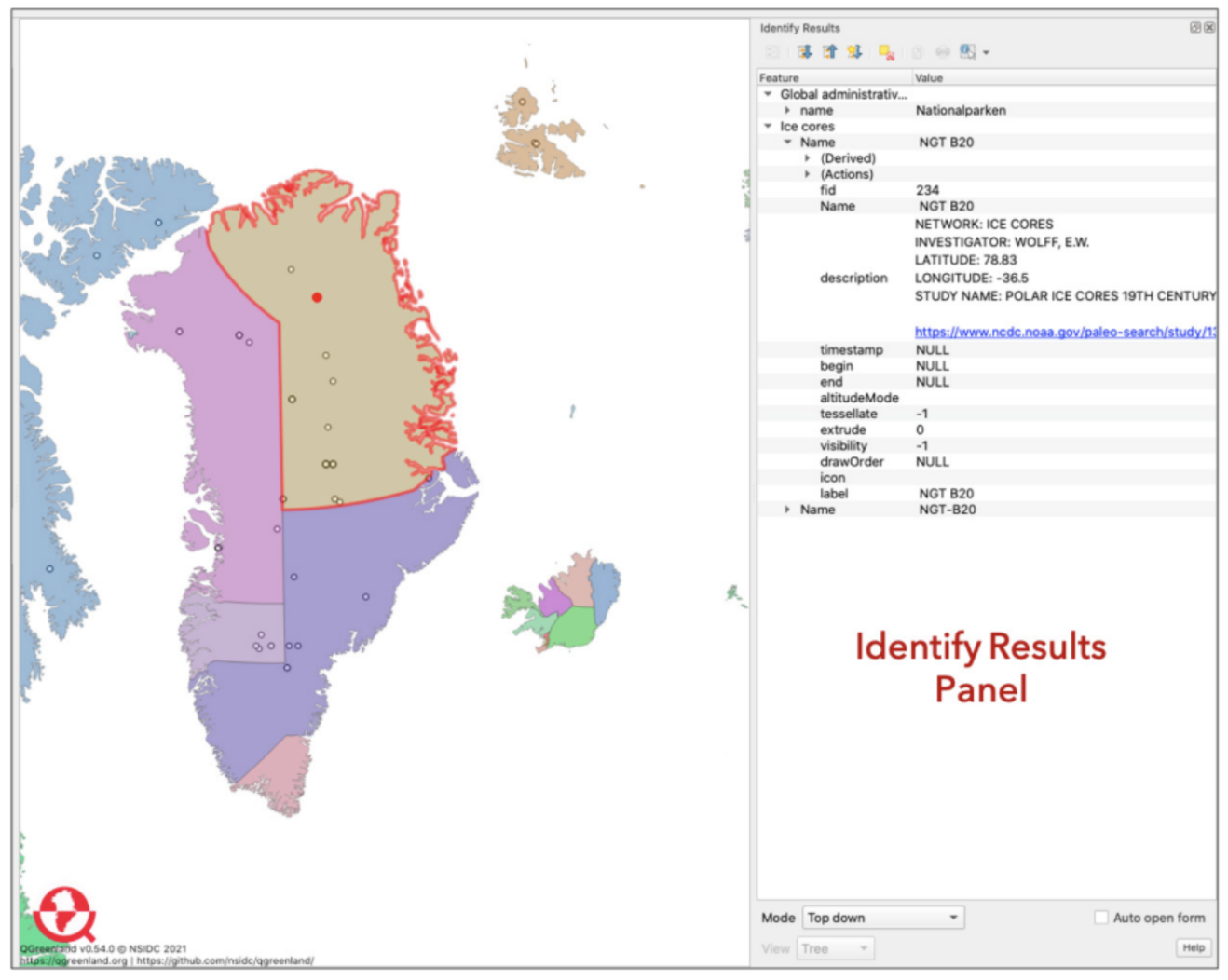
Fig. 7 The Identify Results Panel that shows results from the Identify Features tool.

Measuring Distances, Areas, and Angles

Another useful basic tool in the Attributes Toolbar is the Measuring Tool. The Measuring Tool is a quick and easy way to measure distances between two points or along a line, area of a polygon, or angles between geographic features or locations.

To use the Measuring Tool:

1. Click on the arrow to the right of the Measuring Tool button and choose if you want to measure a line, area, or angle. Regardless of which one you choose, a small window will appear.

2. If you are measuring a line distance, first choose your desired units (e.g. kilometers). Ellipsoidal measurements take into account the spherical shape of the earth and the project’s coordinate reference system. Cartesian measurements assume a flat Earth. For small distances, these numbers will be very similar, but for very large distances they can be very different.

3. Clicking first on one point on the map and then another will draw a line segment whose length will be indicated in the Segments box. You can draw and measure multiple line segments.

4. To clear the segments you’ve drawn, click on New.

5. To measure an area instead of a line with the Measuring Tool, you will follow essentially the same steps for measuring a line distance, except you will click and map out an area on the map instead of drawing line segments.

6. To measure the angle created by three points on the map, click on each of the three points to draw the angle. The second point you click on will serve as the angle’s vertex.

Adding Text Annotations to the Map View

You can add a text annotation anywhere in the Map View using the text annotation tool in the Attributes Toolbar.

To use the Text Annotation Tool:

1. Click on the text annotation button in the Attributes Toolbar.

2. Click on the place on the map where you want the text annotation to go. A small white box will appear.

3. Double click on the box to open a new window where you can write your annotation and choose the font you want to use, among other things (e.g., you can link the annotation to a specific layer).

4. When you are done, click Apply and then Ok to close the window.

5. To delete an annotation, double click on it to open the dialog window, then click Delete.

Editing Layer Symbology

Each QGreenland data layer comes with a predefined symbology (how the layer is visualized in the Map View).

To modify a layer’s symbology:

1. Open the Layer Properties dialog window for the layer you want to edit.

2. Go to the Symbology section and modify the layer symbology as desired. a) For a vector layer, you can choose from a built-in set of QGIS symbols, and/ or can change individual characteristics of the layer’s symbology such as symbol shape, weight, color, size, opacity, and more. b) For a raster layer, you can change the color properties of the grid cells, as well as characteristics like brightness and contrast. The opacity/transparency of a raster layer can be changed in the Transparency tab of the Layer Properties dialog window.

Processing Toolbox

The Processing Toolbox is what makes the QGIS platform a powerful spatial data analysis tool. The Processing Toolbox is a collection of tools and prewritten algorithms that allow the user to perform a wide variety of raster and vector data analyses. For example, the Processing Toolbox contains tools for identifying features in a vector layer that fulfill certain criteria, extracting selected features from a vector layer and saving them as a new layer, and calculating vector and raster layer statistics. The Processing Toolbox can be opened in a new panel to the right of the map view by clicking on the gear icon in the Attributes Toolbar or by going to View -> Panels -> Processing Toolbox Panel in the Menu Bar.

For more in-depth information about the Processing Toolbox see the QGIS User Manual

Examples of using the Processing Toolbox with QGreenland data are given below.

Example 1: Selecting from Vector Layers for Specific Features

Which populated regions in Greenland have more than 5000 people?

1. Open the Processing Toolbox and go to Vector selection -> Select by attribute.

2. Fill in the following parameters: -Input layer = Populated places -Selection attribute = Population 2016 -Operator = ‘>’ -Value = type in ‘5000’ -Modify current selection by = creating new selection These parameters are telling the program to identify all of the populated places in Greenland that have a population greater than 5000.

3. Click on Run. Close the window when processing is complete.

There are a couple of ways to view the selected data points, populated places in Greenland with more than 5000 people. First, you should see the places that meet this parameter highlighted in the Map View (make sure the Populated Places Layer is toggled on). You can also open the Populated places Layer Attribute Table and select Show Selected Features in the bottom left corner. This will hide all records in the Layer Attribute Table except for the ones you selected, the locations with populations greater than 5000 people. If you want to create an entirely new layer based on this feature selection (Population 2016 > 5000), you can do so by either 1) right-clicking on the layer you have just selected from and choosing Export -> Save selected features as…, or by 2) selecting Extract by attribute under Vector selection in the Processing Toolbox.

Example 2: Vector Layer Statistics

What is the total number of people in Greenland’s populated areas? What is the average size of Greenland’s populated areas?

1. Open the Processing Toolbox and go to Vector analysis -> Basic statistics for fields.

2. Fill in the following parameters: -Input layer = Populated places -Field to calculate statistics on = Population 2016 -Statistics = Save to temporary file (or whatever your preference is)

3. Click Run.

The Basic statistics for fields window should automatically switch to a view of the Log where you will see the results for the population basic statistics (Fig. 8). The value ‘MEAN’ will tell you the average size of Greenland’s populated places (702 people). The value ‘SUM’ will tell you the total number of people in Greenland’s metropolitan areas (55,494 people).

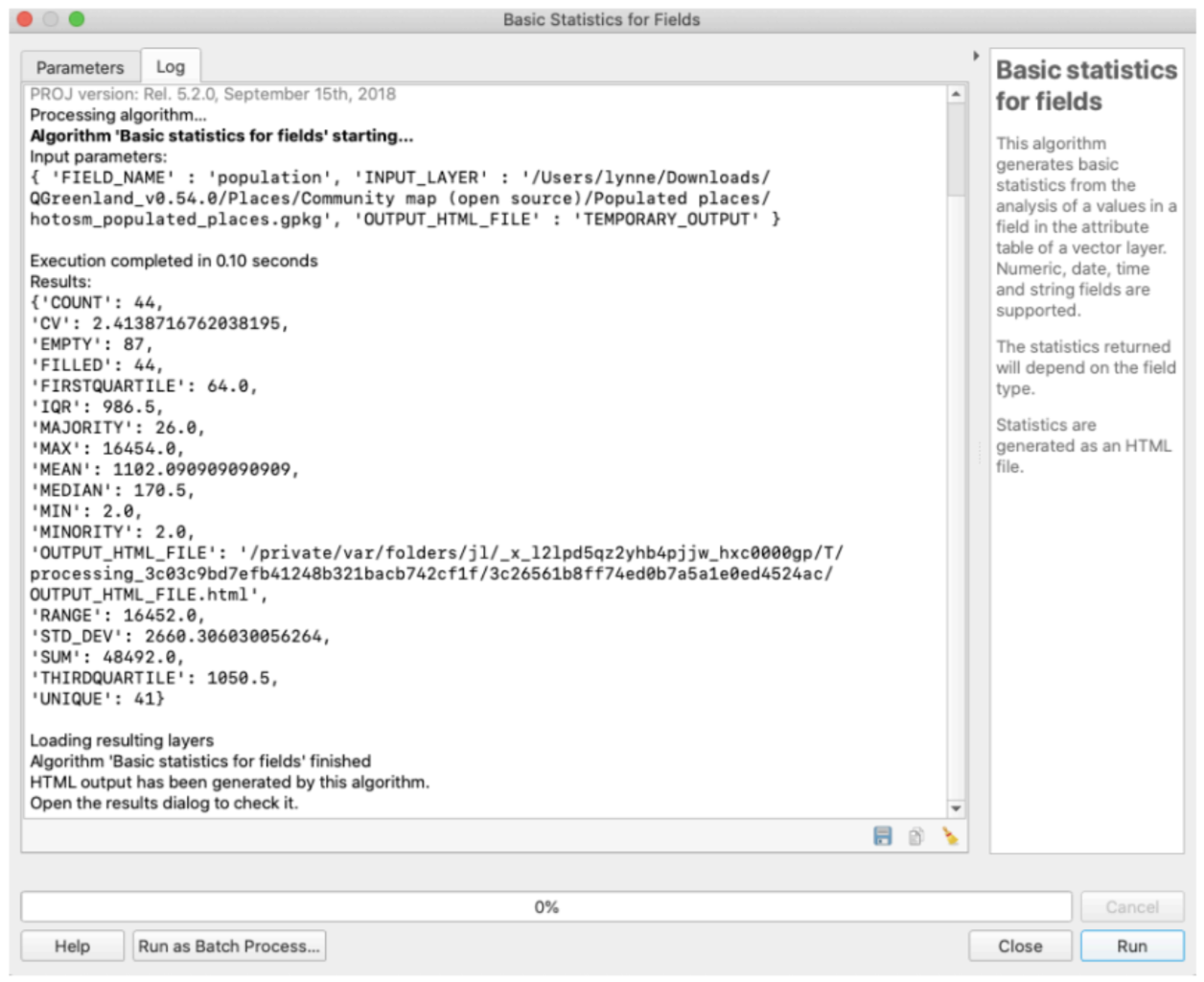
Fig. 8 Results of Example 2: Vector Layer Statistics

Example 3: Simple Raster Analysis

What is a good estimate of the Greenland ice sheet’s volume?

See the Calculate the volume of the Greenland ice sheet tutorial for an example of how to utilize the Raster Surface Volume tool.

Example 4: Using the Raster Calculator

How does the maximum sea ice concentration (%) around Greenland and the surrounding land masses in 2021 compare to the maximum sea ice concentration a decade earlier (2011)?

The Raster Calculator is a tool that allows you to perform calculations on one or more raster layers. For example, if you wanted to convert a raster layer that is in km2 to mi2, you could use the raster calculator. In this example, we are going to use the raster calculator to subtract one layer from another.

Note

There is a different Raster Calculator that can be accessed in the Menu Bar by going to Raster -> Raster Calculator. This calculator is different from the one in the Processing Toolbox used in this example:

1. In the Processing Toolbox, go to Raster analysis -> Raster calculator.

2. In the window that appears, you are going to build a mathematical expression using the layers and operators in the Expression Box: a) In the Layers box, scroll down and double click on the March2021@1 layer (this is the layer for the NSIDC’s sea ice concentration data from March 2021). You should see it show up in the Expression Box in quotations (“ “). b) Either type in the minus (-) symbol or click on it under Operators. It should show up after the layer you just chose. c) In the Layers box, scroll to and double click on the March2011@1 layer. It should show up after the minus sign, again in quotations (Fig. 10). d) For Reference layer, it’s recommended you choose either of the two layers used in the expression. Click on the three dots […] which will open up another window and allow you to choose the reference layer by checking the box next to the layer name.

3. Click Run and close the window.

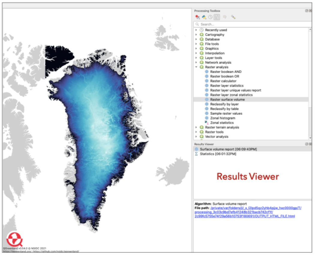
Fig. 9 To view the results of the raster surface volume analysis, click on the link next to ‘File path’ in the Results Viewer Panel below the Processing Toolbox.

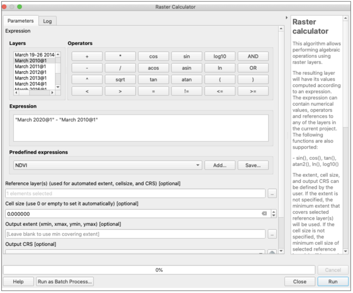
Fig. 10 The Raster Calculator expression for Example 4.

The output layer will appear in the Layers Panel (likely named Output). You can right click on it and rename it if you like. The values next to the colored boxes below the output file (likely black and white boxes) will tell you the minimum and maximum values of the resulting raster layer. In this case, the numbers will be the difference in the maximum sea ice concentration (%) between 2011 and 2021, where positive values indicate an increase between 2011 and 2021 (endmember = +80%), and negative values indicate a decrease (endmember = -95%).